OCaml
An industrial-strength functional programming language with an emphasis on expressiveness and safety
# let square x = x * x
val square : int -> int = < fun >
# square 3
- : int = 9
# let rec factorial x =
if x <= 1 then 1 else x * factorial (x - 1)
val factorial : int -> int = < fun >
# factorial 5
- : int = 120
# square 120
- : int = 14400

The OCaml Compiler has been recognised by SIGPLAN for their prestigious Programming Languages Software Award
Fourteen core OCaml developers are featured for their
significant contributions to the project
Trusted by Industry Leaders
These companies and organisations rely on OCaml every day — along with thousands of other developers. See Success Stories


Why OCaml?
RELIABILITY
Powerful Type Safety Made Simple
OCaml’s lightweight but highly expressive type system catches more bugs at compile time while garbage collection allows you to focus on application logic instead of memory management. Large, complex codebases become easy to maintain and refactor. OCaml empowers you to create mission-critical software with highest security- and safety-requirements in environments with ever-changing requirements!

PRODUCTIVITY
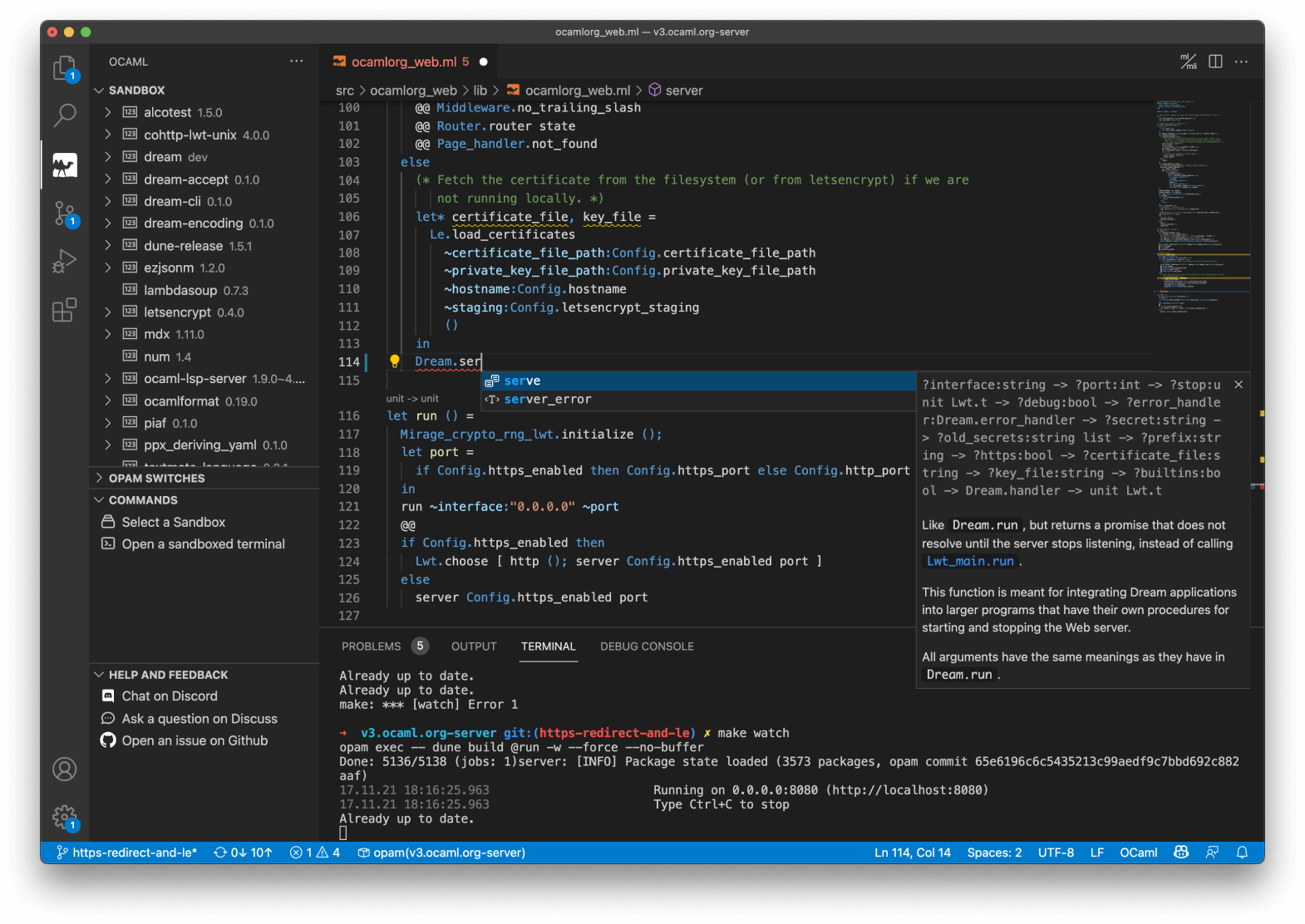
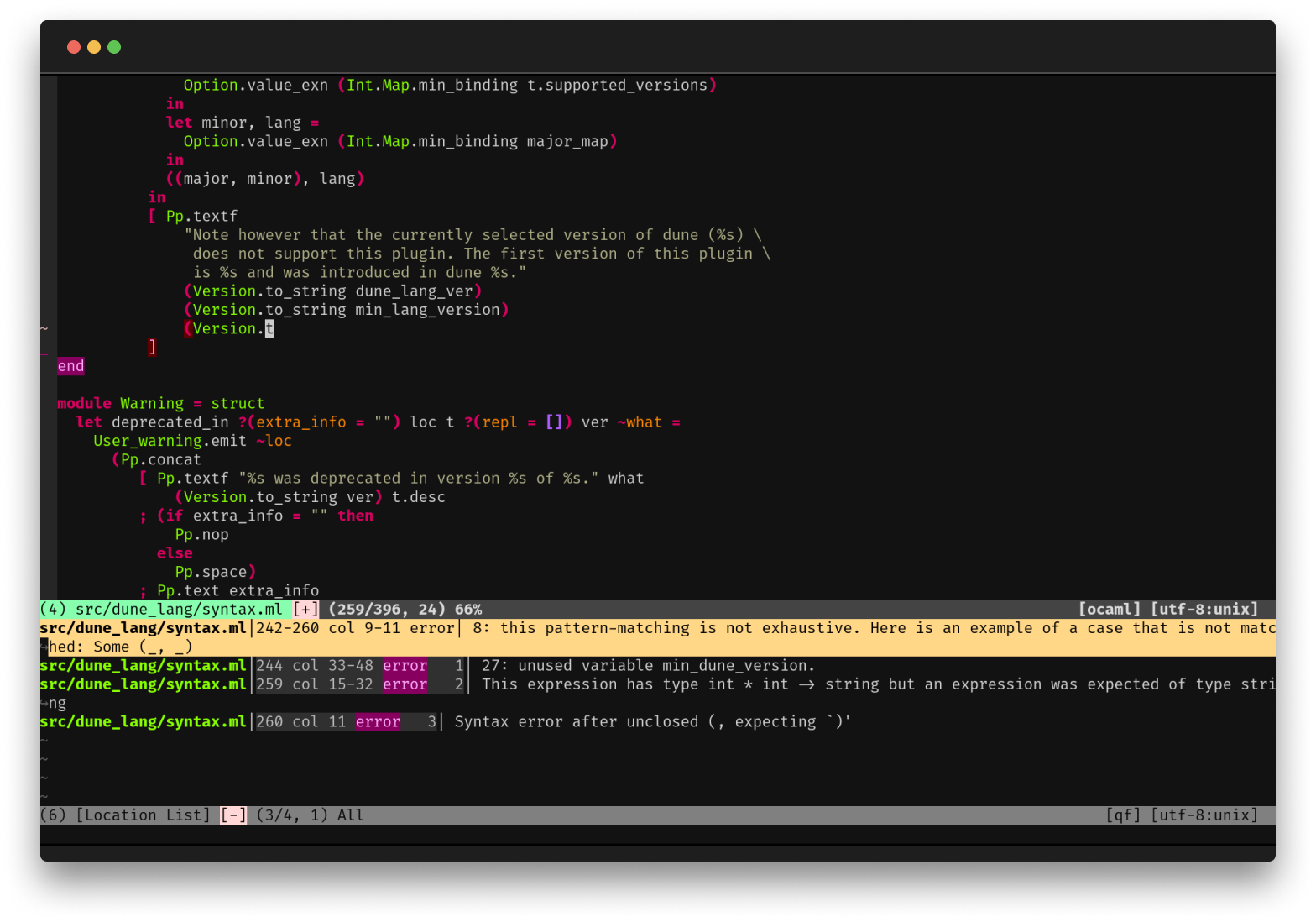
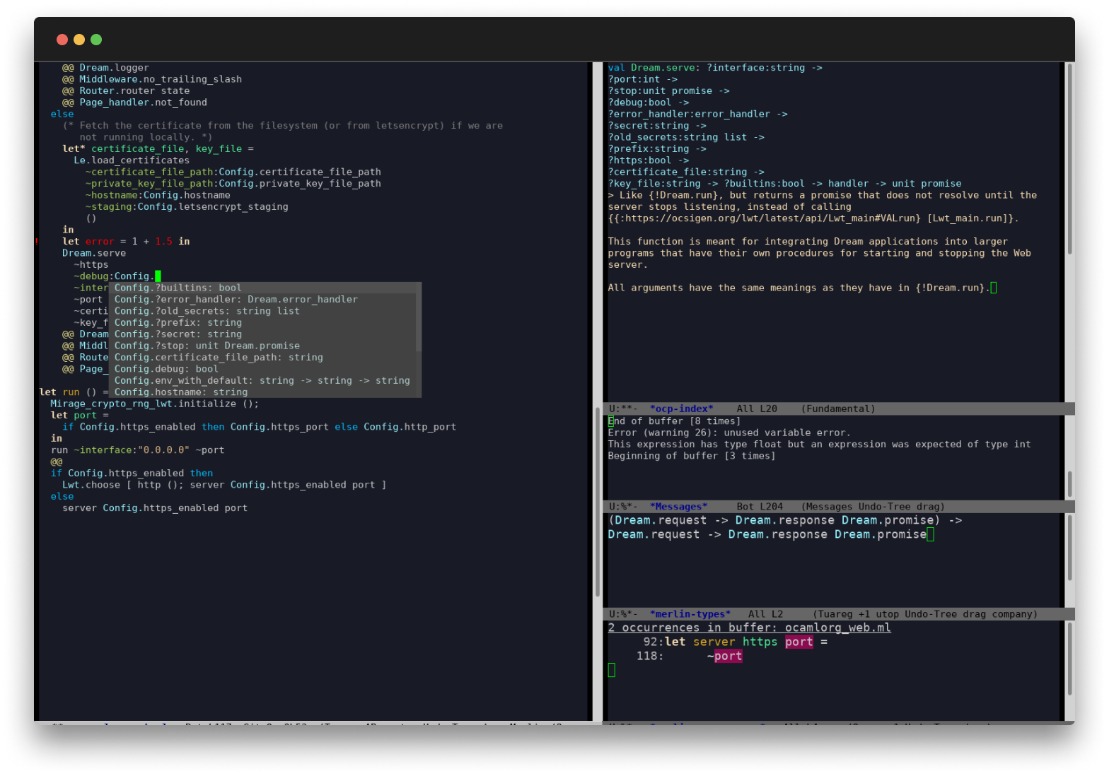
First-Class Editor and Tooling
OCaml comes with deep integrations for VS Code, Vim or Emacs to provide type inspection, autocomplete and more.
Between Opam, a popular package manager; Utop, a powerful interactive REPL; and odoc,
an easy-to-use documentation generator, OCaml programmers have access to a complete, modern developer experience.


PERFORMANCE
Fast Compiler and Applications
OCaml offers great runtime performance without compromising on developer experience: The bytecode compiler generates small, highly portable executables blazingly fast; the native code compiler produces highly-efficient machine code. Despite this focus on performance, the OCaml compiler has always been exceptionally reliable and stable

Exceptionally Robust and Reliable
Despite all this testing, we have never had a single XenServer defect reported from internal testing or from the field that can be traced back to a bug in the OCaml runtime or compiler. (During development we did once find a minor compiler bug, triggered when compiling auto-generated OCaml code with many function arguments, but this was already fixed in the development branch by the time we reported it and so no interaction with the maintainers at INRIA was required.)-- Scott, D. & Sharp, R. & Gazagnaire, T. & Madhavapeddy, A. (2010). Using Functional Programming within an Industrial Product Group: Perspectives and Perceptions. ACM SIGPLAN Notices. 45. 87-92. 10.1145/1863543.1863557.
Releases
Recent Releases
5.3.0 (2025-01-08)
- Syntax for deep effect handlers
- Restored MSVC port
- Re-introduced statistical memory profiling
- More space-efficient implementation of Dynarray
- utf-8 encoded Unicode source files and modest support of Unicode identifiers
- Improved metadata on the pairs of declarations and definitions for merlin.
- Around 20 new functions in the standard library
- Many fixes and improvements in the runtime
- Improved error messages for first-class modules, functors, labeled arguments, type clashes.
- Numerous bug fixes
5.2.1 (2024-11-18)
- Bug fixes for 5.2.0
Changelog
Releases & Updates
Compiler and Platform Tools
# Emacs Integration for OCaml LSP Server: Introducing ocaml-eglot ## TL;DR `ocaml-eglot` provides...
See full changelogThe Dune Team is happy to announce the release of Dune `3.20.1`. This release introduces some mino...
See full changelogThe Dune Team is happy to announce the release of Dune `3.20.0`. This release contains some import...
See full changelogUsers of OCaml
OCaml is used by thousands of developers, companies, research labs, teachers, and more. Learn how it fits your use case.
For Educators
With its mathematical roots, OCaml has always had strong ties to academia. It is taught in universities around the world, and has accrued an ever-growing body of research. Learn more about the academic rigor that defines the culture of OCaml.
Learn moreFor Industrial Users
OCaml's powerful compile-time guarantees and high performance empower companies to provide reliable and speedy services and products. Learn more about how OCaml is used in the industry: explore success stories and discover companies that use OCaml.
Learn moreCurated Resources
Get up to speed quickly to enjoy the benefits of the OCaml programming language across your projects.
Getting Started
Install OCaml, set up your favorite text editor and start your first project.
Language Manual
Read the reference manual of the language and documentation on the compiler.
Books
Discover OCaml books from expert programmers and researchers - from beginner level to advanced topics.
Standard Library
Searchable API documentation.
Exercises
Learn OCaml by solving problems on a variety of topics, from easy to challenging.
Papers
Explore papers that have influenced OCaml and other functional programming languages.
OCaml Packages
Explore thousands of open-source OCaml packages with their documentation.